A Monte Carlo simulation does not show one end date, it shows a probability. With the new MCP server in Merlin Project, you ask Claude in a single sentence to read your plan and compute 10,000 project runs. Here is how to do it.
A Monte Carlo simulation translates uncertainty into probability. Instead of a single date you get a distribution of possible finish dates. With the MCP server in Merlin Project, this no longer requires a specialist add-in or laboriously maintained estimates; a single sentence to Claude is enough.
What a Monte Carlo simulation is exactly and why it beats the critical path is explained in our guide to Monte Carlo in project management. This is about putting it into practice: how you actually compute the simulation with Merlin Project and the MCP server.
Merlin Project and the MCP Server
Merlin Project ships with an MCP server. MCP stands for Model Context Protocol, an open standard that gives AI assistants a structured and secure connection to external applications. The server runs locally on your Mac and is not reachable remotely; it uploads nothing on its own and discloses only what the AI actively queries. What the AI reads, however, it processes at the respective provider: with a cloud client like Claude, the plan data that is read goes to its API. You keep control over which project you release, fully in the spirit of digital sovereignty. You activate it per project via the "AI Tools" button in the document's toolbar. The full setup for Claude Desktop, Claude Code and other clients is in the MCP documentation.
Read Access Is Enough
The MCP server currently offers read-only access to project data. For a Monte Carlo simulation, this is exactly right: the client can only read the plan, nothing in the plan itself can be changed. The simulation reads the plan just once; the entire stochastic computation runs outside Merlin. Nothing is written back into the live plan. Your project structure remains the untouched single source of truth, and you can simulate as often as you like and on any plan version.
From the plan the AI reads three things. First, the tasks with their planned duration. Second, the network logic, that is the dependencies between predecessor and successor, including the link type and float. Third, the location of the uncertainty, that is which task a risk is attached to. The network logic is the core: without the dependency edges you would only add durations together, instead of computing a network diagram.
The Crux: the Uncertainty Is Not Yet in the Plan
Merlin stores a planned duration per task and later an actual value, but no native three-point estimate. There are three ways to solve this:
- Custom fields. You add O and P as user-defined fields in the template and read them along via MCP. The cleanest solution, if you control the template.
- Global uncertainty band. Planned duration plus or minus X percent as a triangle or PERT, scaled by phase or task type as needed.
- Hybrid. Annotated risk tasks get their own band, the rest a default.
Whichever route you choose: show transparently where the uncertainty comes from. That is exactly what makes a simulation credible.
The Agentic Process, and the Mistake You Must Avoid
Here lies the most common misconception: Claude does not run through the 10,000 iterations itself. No language model draws 10,000 random samples in its head. That would be not only token-intensive but statistically worthless, because language models are poor random generators. The iterations belong in code.
The trick is not "Python script versus MCP client," but code execution by the client. The process has three steps:
- Read. Claude calls the read tools of the Merlin MCP server and fetches tasks, durations and dependencies.
- Compute. Claude writes the simulation for itself in a few lines of numpy and runs it, as part of the answer. This requires a client with code execution, such as Claude Code; a plain chat window without code execution cannot run the iterations. Per iteration the model draws one duration for each task, runs through the network diagram in topological order (respecting predecessors and lags) and takes as the project end the latest finish of all end nodes.
- Explain. Claude returns the S-curve, P50, P80 and P90 as well as a tornado diagram and interprets the result in plain language.
From your point of view the narrative is simple. You ask a question in natural language:
Read the active project from Merlin Project and simulate 10,000 possible
project runs. For each task, assume the planned duration plus/minus 20 percent
as a PERT distribution. Show me the S-curve and the dates for P50, P80 and P90.
Claude reads the plan, computes and shows you the probability curve. The code behind it is an implementation detail, not a learning step. It is like a calculator: you use it instead of multiplying in your head.
By the way, it is not the iterations that are token-intensive (in code they are practically free), but pulling a 300-line task list into the context. So for getting started the rule is: a deliberately small, clean example plan with 15 to 25 tasks. That is large enough for path convergence and an interesting tornado, and small enough that the whole conversation fits on one screen.
The Result from 10,000 Runs
This is what Claude's answer to the prompt above looks like, computed on a small construction-project plan. Claude connects to the active document, reads tasks, links (26 finish-to-start, one start-to-start) and the calendar (Monday to Friday, 8 hours per day), rebuilds the network and validates it against the planned end date. The model reproduces it exactly: 60 working days, that is Aug 21, 2026. Then the 10,000 runs go through.

This example project comprises only around two dozen tasks, whose schedule is determined by a long, serial chain. That is why the spread between P10 and P90 is deliberately narrow at about one week; larger or more branched projects typically scatter considerably further.
| Confidence | Date | Versus plan (Aug 21) |
|---|---|---|
| Planned date | Aug 21, 2026 | roughly 49 percent chance of hitting it |
| P50 | Aug 24, 2026 | plus 1 working day |
| P80 | Aug 25, 2026 | plus 2 working days |
| P90 | Aug 26, 2026 | plus 3 working days |
The range across all 10,000 runs reaches from Aug 17 at the earliest to Sep 1 at the latest.
The reading is unambiguous: the planned date is a 50/50 date. In roughly half of the runs it is held, in the other half it is missed. That is the typical finding, because deterministic planning almost always lands on the optimistic P50, not on a dependable delivery date. Whoever wants to commit with 90 percent certainty communicates Aug 26, that is around three working days of buffer.
Claude discloses its own assumptions: here the planned duration served as the most likely value, with O at −20 percent and P at +20 percent as a symmetric PERT-beta distribution. With the real, in part asymmetric three-point estimates from the plan, the right tail would be longer and P90 later. The discrete risk events, the supplier failure and the structural engineer dropout, are not modeled here; this was pure duration spread. Those are exactly what we work through in the next two examples.
Example A: the Supplier Comparison
The strongest example answers a decision question, not just a forecast question. Picture a task that depends on a delivery. Supplier A delivers on time in a portion of cases, otherwise with a few days of delay. The denominator matters here: 10 late out of 100 deliveries is a different risk than 10 out of 15. This is exactly where Monte Carlo shows its strength, because it does not compute with made-up assumptions, but translates lived delivery history into a forecast.
The real value lies in the money-versus-risk trade-off. Supplier A is cheaper but less reliable; supplier B is more expensive but stable and costs 4,000 € more. Is the surcharge worth it? Management understands this question immediately, and Monte Carlo answers it with a number instead of a gut feeling.
You ask Claude a question like this in a single sentence:
Task 19 "material installed" depends on a delivery. Supplier A delivers on time
in 85 percent of cases by experience, otherwise with a 10-day delay. Simulate how
this affects the finish date, and compare it with supplier B, who always delivers
on time but costs 4,000 € more.
Claude attaches the risk switch to the delivery and computes both suppliers with the same random draws (common random numbers), so that the difference depends cleanly only on the delivery. The result is strikingly clear (wd stands for working days):
| Confidence | Supplier A (85% on time, otherwise +10 wd) | Supplier B (always on time, +4,000 €) |
|---|---|---|
| P50 | Aug 21, 2026 | Aug 21, 2026 |
| P80 | Aug 25, 2026 | Aug 25, 2026 |
| P90 | Aug 25, 2026 | Aug 25, 2026 |
| Planned date held | 50.5% | 50.5% |
| Finish-date slip from A | 0.00% | reference |
In none of the 10,000 runs does the unreliable supplier A shift the finish date. The two distributions are congruent. The reason is in the plan: task 19 "material installed" depends on two predecessors, the delivery and the roof on the critical path. The roof is systematically finished later, so "material installed" waits on the roof anyway, not on the facade delivery. Between delivery and installation there is a median buffer of 21 working days, and a good 17 even in the most compressed run. A delay of 10 working days never reaches that limit.
You can see this best in the sensitivity: how large would the delay even have to become to move the finish date?

Only above this buffer edge, beyond roughly 17 to 21 working days, does anything start to break through at all: at 25 days 7 percent of runs slip, at 30 days around 15. The cost decision is thus clear. Under these assumptions, the 4,000 € for supplier B buy zero schedule gain; the expected avoided delay is 0.0 working days. From a pure schedule perspective, supplier A is the rational choice; the money would be paid for a risk that the plan already carries through its buffer. B only pays off once an assumption shifts: when the delay becomes much larger than 10 days (an import container instead of a regional delivery), when the shell construction finishes much earlier and the buffer shrinks, or when the facade strand carries its own intermediate dates backed by contractual penalties. That is exactly what a purely deterministic plan could never show.
An honest footnote: the two examples are separate simulation runs with their respective risk switches. One day of deviation in the base date compared to the S-curve further up is normal sampling noise, not a contradiction. Monte Carlo estimates a distribution; it is not a calculator with fixed decimal places.
Example B: the Resource Dropout
The second example turns a different dial: not the duration, but a discrete event. A key resource could drop out, here the structural engineer, who works on two tasks, the structural design early in the project and the structural acceptance late. Does the engineer drop out, and if so, when does it hit harder?
Simulate my project for three cases: resource "structural engineer" does not drop
out, drops out in week 3 for 10 days, drops out in week 8 for 10 days. Show me
P50/P80/P90 for each and which dropout timing hits the finish date hardest.
Again Claude computes all three cases with the same random draws, so that the differences depend cleanly only on the dropout:

| Case | P50 | P80 | P90 | Shift |
|---|---|---|---|---|
| No dropout | Aug 21, 2026 | Aug 25, 2026 | Aug 25, 2026 | base |
| Early dropout (structural design) | Sep 4, 2026 | Sep 8, 2026 | Sep 8, 2026 | +10 wd |
| Late dropout (structural acceptance) | Sep 2, 2026 | Sep 4, 2026 | Sep 7, 2026 | +8 wd |
Both dropouts miss the planned date for sure, the chance of hitting it drops from 50 to 0 percent. What is interesting is the difference: the early dropout hits harder. In 100 percent of runs it shifts the finish date further than the late one, on average by 2 working days. The reason is again the buffer situation, not the timing as such. The structural design lies fully on the critical path, without buffer; its ten dropout days break through 1:1, a clean plus 10 working days in every run. The structural acceptance, by contrast, draws a small remaining buffer from a parallel strand that absorbs two of the ten days before it becomes the binding task itself. That leaves plus 8 working days.
That is the solid lesson from example B: an equally long dropout costs a different amount depending on how much buffer the affected task has. Cover, lead time and reserve belong first to the resources on the critical path that have no buffer.
Critical Path Versus Buffer: the Shared Point
Both examples say the same thing at their core: it is not the risk alone that decides, but where it sits in the network diagram. The same delay costs nothing on a task with buffer and everything on the critical path. Monte Carlo does not show "delay is bad," but when a risk breaks through and when the plan absorbs it. That is why the cheap supplier in example A was the rational choice and the early dropout in example B the expensive one: in the first case a buffer catches the risk, in the second it is missing. How to adjust the critical path in Merlin Project deliberately is shown by this tutorial.
Try It Out
The technique behind Monte Carlo is decades old. What is new is how easy it has become. With Merlin Project's MCP server, your plan is already in a form that an AI can read and compute. A specialist add-in with its own data maintenance becomes a single sentence to Claude.
If you already use Merlin Project, activate the MCP server for a project and ask your first question. The setup is in the MCP documentation. If you do not know Merlin Project yet, get to know it on the product page or download it directly to try it out.
And nobody has to write up the results by hand. On request, Claude bundles the whole run into a finished report for your stakeholders. The full report for this example project shows how that looks: Download the Monte Carlo report (PDF, in English).
If you have any questions about this blog article or would like to discuss it, we look forward to your contribution in our forum.
Frequently asked questions
Do I need programming skills for a Monte Carlo simulation with the MCP server?
No. You ask your question in natural language, and Claude writes the simulation itself in code and runs it. All you need is a client with code execution, such as Claude Code.
Does the simulation write changes back into my Merlin Project plan?
No. Read access alone is enough for the simulation. The AI reads the plan once, computes outside Merlin and writes nothing back into the live plan. Your project structure stays untouched.
Which client do I need to compute the simulation?
An MCP client with code execution, for example Claude Code. A plain chat window without code execution cannot run the 10,000 iterations.
Is my project data safe with the MCP server?
The MCP server itself runs locally on your Mac and is not reachable remotely; it uploads nothing on its own. What the AI reads, however, it processes at the respective provider: with a cloud client like Claude, the plan data that is read is transmitted to its API. You release per project what the AI may see, and nothing is written back into the plan.
How large should my plan be to get started?
A deliberately small plan with 15 to 25 tasks is ideal: large enough for path convergence and a meaningful tornado, small enough that the whole conversation stays manageable.